Quick Start
Overview
The main purpose of cronus is to facilitate large-scale Bayesian Inference (e.g. MCMC or NS) in modern
super-computing environments. cronus utilises MPI to efficiently distribute the tasks to multiple
nodes. Another important feature of cronus is its integrated and automated suite of Convergence Diagnostics.
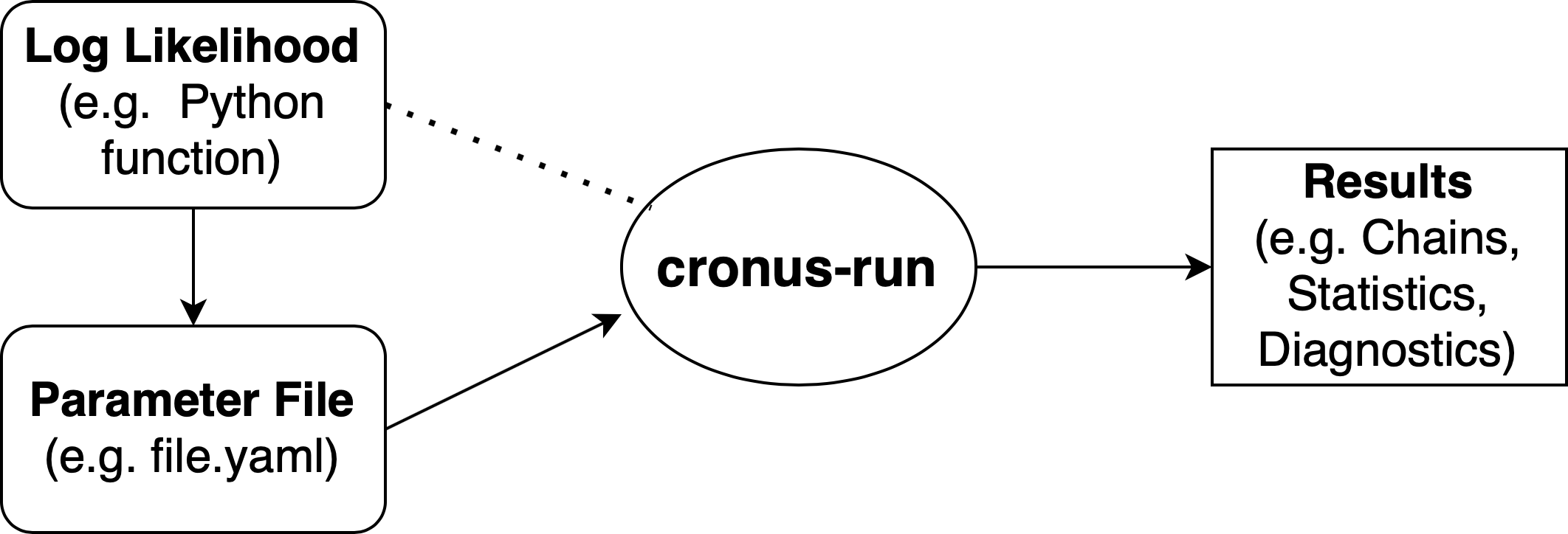
Before we go into detail about how to use cronus let us first discuss the way it works in a higher level.
cronus accepts as an input a parameter file that specifies the following:
- The Python file that contains the definition of the Log Likelihood function,
- A set of priors and/or fixed values for the different parameters of the model that enters the Log Likelihood function.
Note
The Paremeter file can also be used to specify some additional optional information, like:
- A set of parameters that configure the MCMC/NS sampler (e.g. number of walkers), those are usually trivial to define.
- A few threshold values for the Convergence Diagnostics,
- The path/directory for the results to be saved in.
For more information about this please read the Advanced Use page.
Once a parameter file is provided, cronus efficiently distributes the sampling tasks to all available CPUs and runs
until Convergence is reached. The results are saved iteratively so that the researcher can monitor the progress.
Let us present here a simple example that will help illustrate the basic features and capabilities of cronus.
Log Likelihood Function
The first thing we need to do is to create a Python file in which we define the Log Likelihood function. There is
no real restricton to this. The model itself can be computed in any programming language (e.g. C, C++, Fortran) and
the Log Likelihood can be a Python wrapper for this. In this example we will define a strongly-correlated
5-dimensional Normal distribution.
import os
os.environ["OMP_NUM_THREADS"] = "1"

import numpy as np

ndim = 5

C = np.identity(ndim)
C[C==0] = 0.95
Cinv = np.linalg.inv(C)

def log_likelihood(x):
    return - 0.5 * np.dot(x, np.dot(Cinv, x))
We then save the file as logprob.py.
Note
The important thing to note here is that the function accepts a single argument x. If your Log Likelihood
requires more than one argument (e.g. data, covariance, etc.) we recommend to make those global like we did with
the ivar array in the aforementioned example.
Note
Some builds of NumPy (including the version included with Anaconda) will automatically parallelize some
operations using something like the MKL linear algebra. This can cause problems when used with the
parallelization methods described here so it can be good to turn that off (by setting the environment
variable OMP_NUM_THREADS=1, for example).
import os
os.environ["OMP_NUM_THREADS"] = "1"
Parameter File
The next step is to create the parameter file that we will call file.yaml:
Likelihood:
  path: logprob.py
  function: log_likelihood

Parameters:
  a:
    prior:
      type: uniform
      min: -10.0
      max: 10.0
  b:
    fixed: 1.0
  c:
    prior:
      type: normal
      loc: 1.0
      scale: 1.0
  d:
    prior:
      type: normal
      loc: 0.0
      scale: 2.5
  e:
    prior:
      type: normal
      loc: -0.5
      scale: 1.0
You can see the following sections in the parameter file:
- The
Likelihoodsection which includes information about the path of the Log Likelihood function (i.e. both the directory/filename and the name of the function). - The
Parameterssection which includes the priors of fixed values for each parameter of the model.
For more information about these and additional options in the parameter file please see the Advanced Use page.
Run cronus
To run this example go the directory where you saved file.yaml and do:
$ mpiexec -n 8 cronus-run file.yaml
Here we used 8 CPUs.
Results
After a few seconds, an output directory will be created containing the following files:
chains/run1
         ├── chain_0.h5
         ├── chain_1.h5
         ├── IAT_0.dat
         ├── IAT_1.dat
         ├── GelmanRubin.dat
         ├── MAP.npy
         ├── hessian.npy
         ├── para.yaml
         ├── results.dat
         └── varnames.dat
All but the results.dat file will be created shortly. The files will iteratively be updated every few iterations.
Once the sampling is done, the results.dat file will be added to the list.
Let’s have a look at what each of those files contains:
- The
chain_x.h5files contain the actual MCMC samples. - The
IAT_x.datfiles contain the estimated Integrated Autocorrelation Time (IAT) for each and parameter. This is a measure of how independent the chain samples are (i.e. the lower the IAT the better). - The
GelmanRubin.datfile contains the Gelman-RubinR_hatdiagnostic for each parameter. - The
MAP.npyfile contains the Maximum a Posteriori (MAP) estimate. - The
hessian.npyfile contains the Hessian matrix evaluated at the MAP. - The
para.yamlfile is a copy of the original parameter file with some extra information explicitly described. - The
results.datfile includes a summary of the results (e.g. mean, std, 1-sigma, 2-sigma, etc.). - The
varnames.datfile contains a list of the parameter names.
Note
If we can open the results.dat file using a text editor we will see the following:
| Name   |      MAP |     mean |   median |      std |   -1 sigma |   +1 sigma |   -2 sigma |   +2 sigma |     IAT |     ESS |   R_hat |
|--------+----------+----------+----------+----------+------------+------------+------------+------------+---------+---------+---------|
| a      | 0.885898 | 0.881579 | 0.879316 | 0.304584 |  -0.301652 |   0.308398 |  -0.609184 |   0.609584 | 6.82365 | 4044.76 |  1      |
| c      | 0.891147 | 0.879663 | 0.881513 | 0.298963 |  -0.301561 |   0.293607 |  -0.603484 |   0.59629  | 6.87625 | 4013.82 |  1.0003 |
| d      | 0.878582 | 0.880138 | 0.881647 | 0.307091 |  -0.311894 |   0.302304 |  -0.617898 |   0.611955 | 6.814   | 4050.48 |  1.0006 |
| e      | 0.818762 | 0.807181 | 0.807153 | 0.297321 |  -0.29532  |   0.294845 |  -0.593549 |   0.597654 | 6.5086  | 4240.54 |  1.0002 |
Now let’s see how we can easily access this information using cronus.
The first thing we want to do is read the chains using the read_chains module of cronus:
import cronus

results = cronus.read_chains('chains/run1')

print(results.Summary)
This will print the contents of the results.dat file.
We can easily create some plots by running:
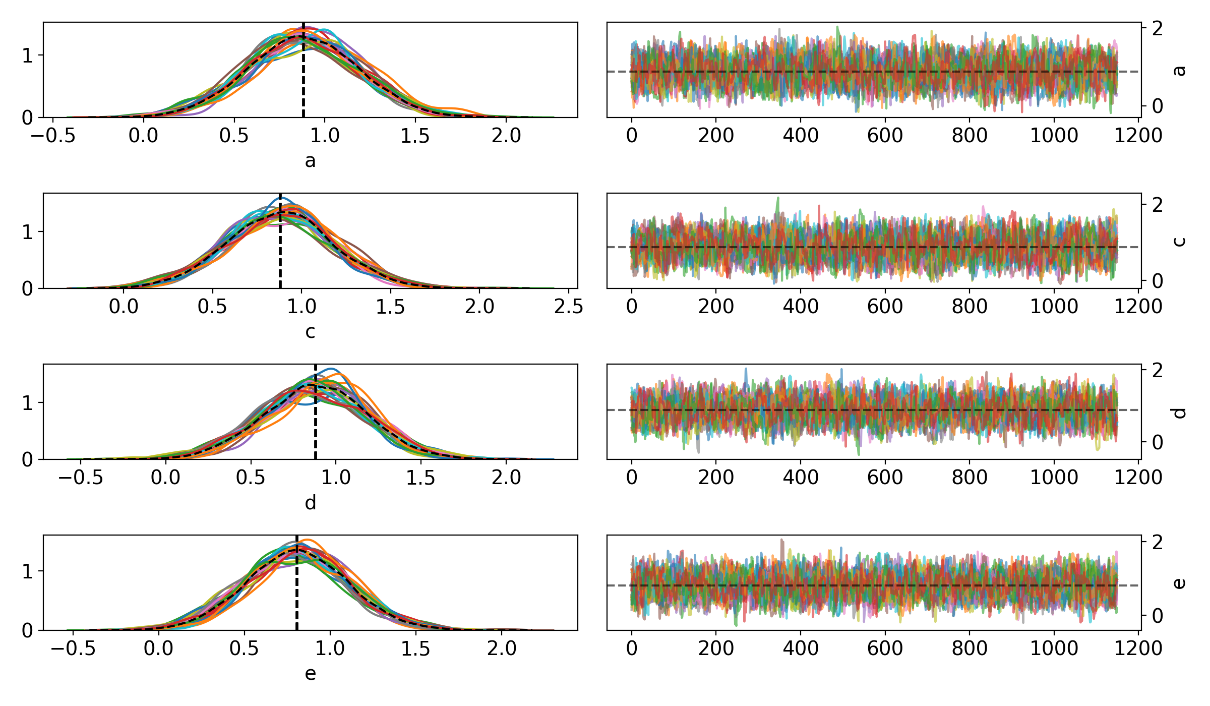
cronus.traceplot(results)
to get the following traceplot:
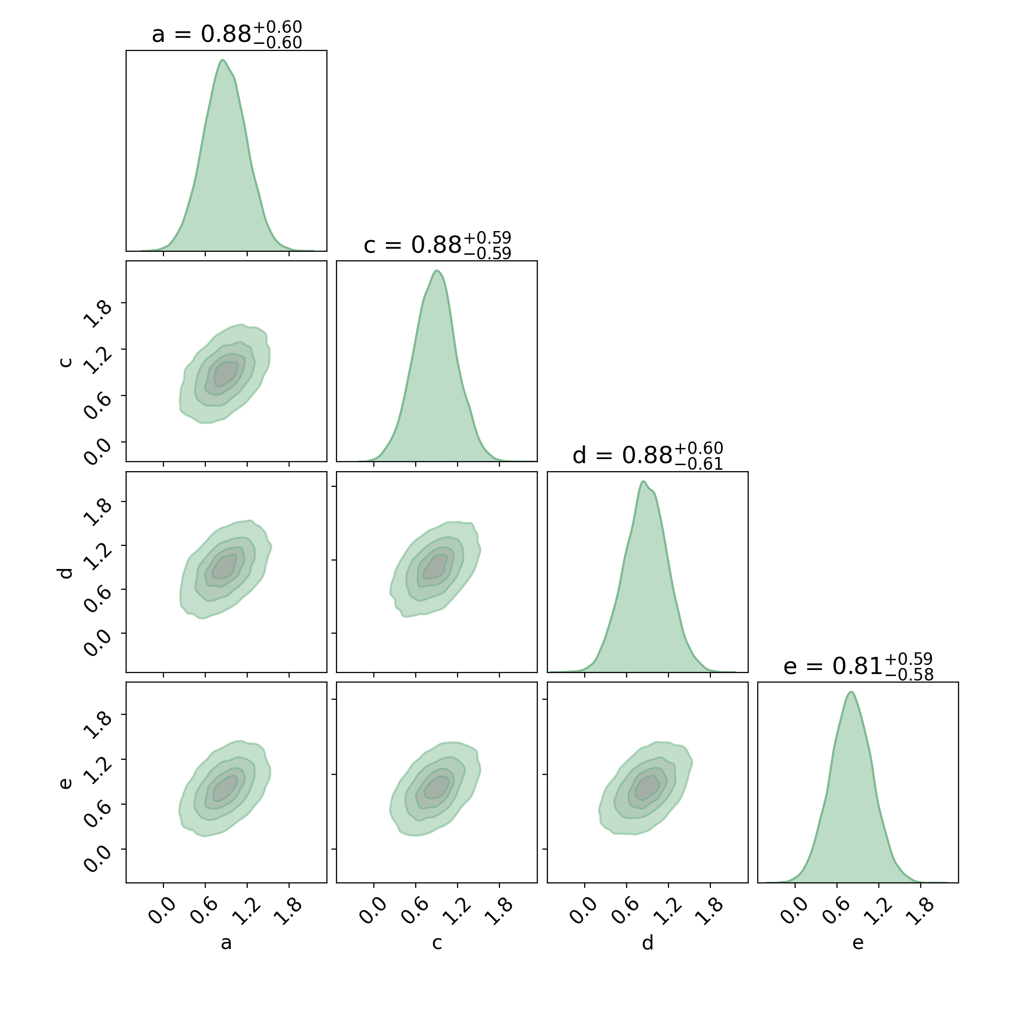
Or, run the following to get a cornerplot:
fig, axes = cronus.cornerplot(results.trace, labels=results.varnames)